tubebench | Woongji Kim

Synopsis

Commercial impedance-tube systems, especially four-microphone tubes for transmission loss and transfer impedance, are expensive and tied to their vendor’s hardware, so many labs build their own. But a home-built tube solves only the hardware half: run by hand across separate instruments and scripts, settings drift, channels get swapped, and calibrations stop matching the data. Instrument control is what turns a do-it-yourself tube into a measurement system.

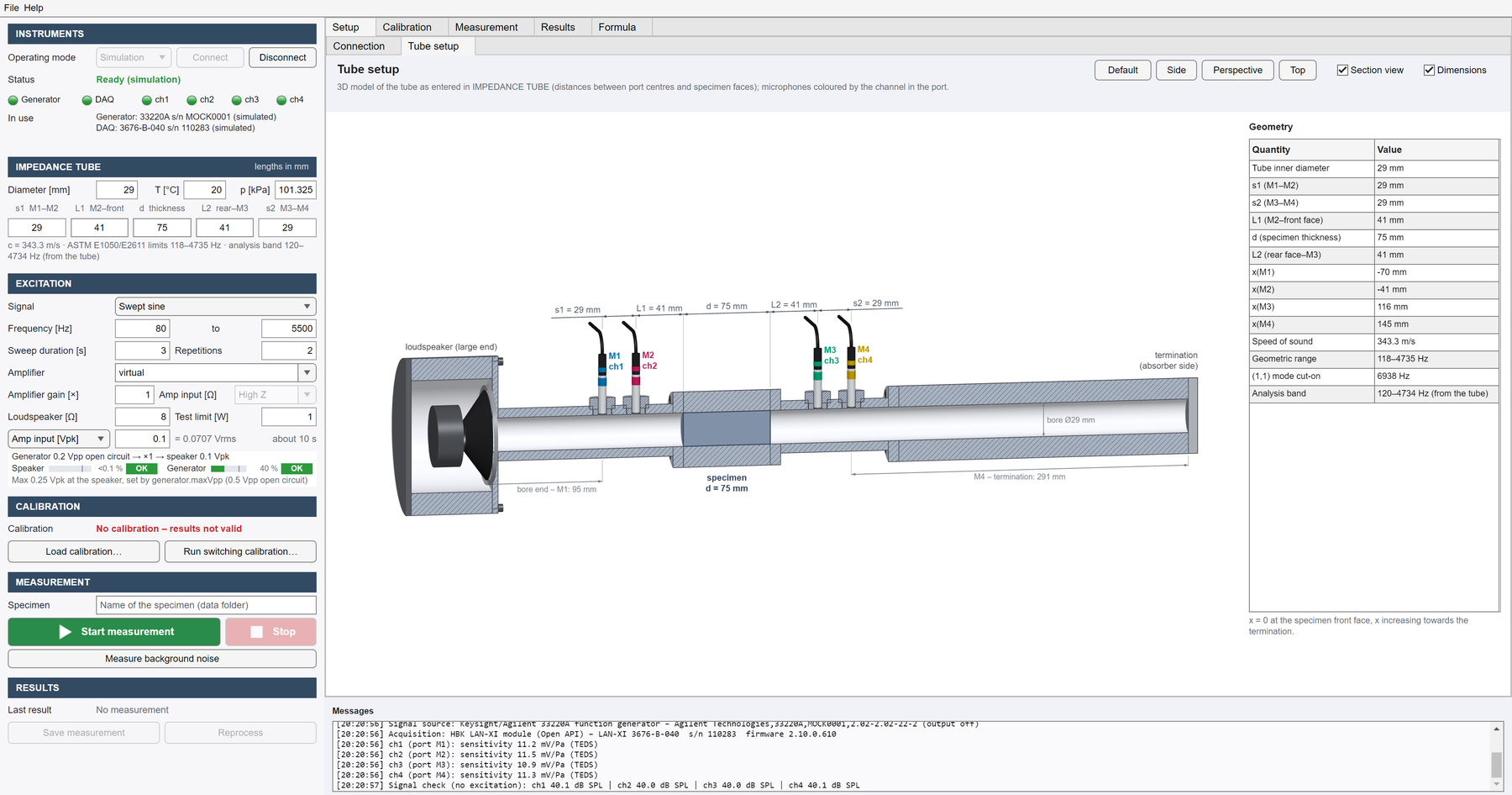
tubebench does this in one window. It drives the signal generator and the acquisition, guides the microphone calibration, and computes the specimen’s properties after ASTM E2611¹, flagging every frequency line it cannot trust. It runs on general-purpose instruments, takes new ones through a driver interface, includes a virtual tube for trying it without hardware, and is open source.

The tubebench window: instrument, tube, excitation, calibration and measurement controls on the left, and a 3D section of the four-microphone impedance tube on the right

The tubebench window: the controls follow the workflow from top to bottom, and the 3D tube follows the geometry entered.

Method	Four-microphone transfer-matrix method (ASTM E2611)
Results	Reflection, transmission, transmission loss, transfer impedance, transfer matrix
Excitation	Swept sine, stepped sine, random noise
Instruments	Keysight 33220A, HBK LAN-XI; others through drivers, guided by a Claude Code skill
Platform	MATLAB R2022b, Signal Processing Toolbox
Licence	MIT · github.com/kimwoongji/tubebench

Measurement chain

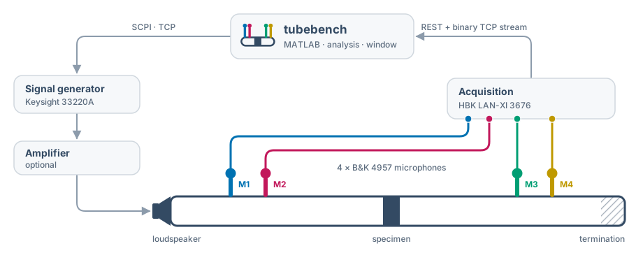
tubebench drives the generator over SCPI and reads four microphones through the acquisition module.

The generator and the acquisition need no shared clock. All four channels are sampled together, so dividing each by a reference channel cancels the unknown drive spectrum $S(f)$; the remaining complex gain ratio $C_k$, amplitude and phase, is removed by the calibration below.

$$ H_k^{\,m} = \frac{Y_k}{Y_{\mathrm{ref}}} = C_k\,H_k $$

As in the automated field characterization system, safety checks are part of the sequence: the output level is read back before the generator is switched on, and configured limits refuse unsafe settings.

Adapting to other labs

Another lab’s tube rarely comes with the same instruments. tubebench talks to hardware only through drivers, so supporting a new signal generator or acquisition module, including NI DAQ devices and audio interfaces, means writing one driver class; the session, calibration, analysis and window stay unchanged.

In Claude Code, the /add-instrument skill walks a lab through it:

Manual first: start from the instrument’s programming manual; commands are never guessed.
Suitability check: confirm the instrument can do what the measurement needs before writing any code.
Driver, model and tests: build them from templates, then test everything in simulation.
Hardware, step by step: verify on the real instrument one step at a time, with the operator present and the output off first.

Switching calibration and validity

Switching calibration on the virtual tube.

The gain and phase mismatch between microphones is measured in place by swapping them between ports: twelve guided steps, closed by an automatic empty-tube check. Every frequency line then gets a verdict, and lines that the geometry, calibration, signal quality or termination cannot support are masked, with the reason shown.

Verification

To check the whole chain against an independent reference, a 3D-printed resonator cell was measured with one load and with two loads (ASTM E2611) on the same mount, and compared with a 3D finite-element model with thermoviscous losses.

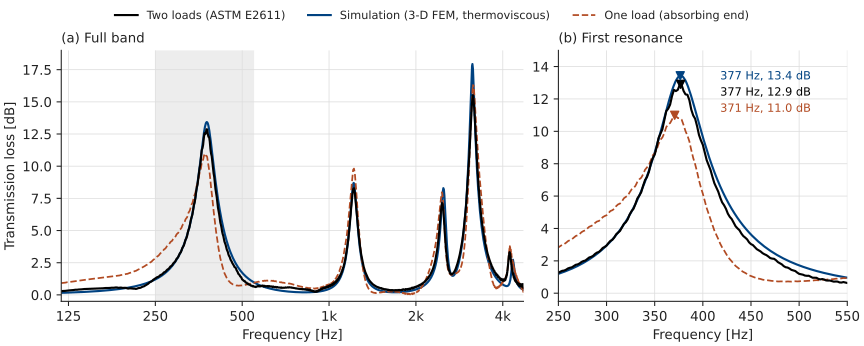
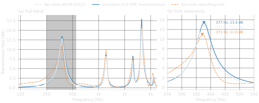
Transmission loss of the cell: (a) over the tube's band, (b) around the first resonance (shaded in a).

With two loads, the measured transmission loss follows the simulation: 377 Hz and 12.9 dB at the first resonance against 377 Hz and 13.4 dB, and the other resonances lie within 3 % of the simulated frequencies, though up to 2.4 dB lower above 2 kHz. The one-load curve, the transmission coefficient with the absorbing end alone, is biased by that end’s reflection ($\lvert R \rvert \approx 0.5$ near 400 Hz) and peaks at 371 Hz and 11.0 dB; the two-load transfer matrix removes that dependence. A repeat of the first load reproduced the transfer matrix to 3 % (median), so the specimen had not moved, and tubebench flagged the lines it could not trust.

Development Contributions

Instrument control for a home-built four-microphone tube: the full ASTM E2611 workflow in one application.
No shared clock needed between generator and acquisition.
Self-qualifying results: a validity verdict for every frequency line.
Two-load transfer matrix (ASTM E2611), with a repeat of the first load to show that the specimen did not move.
Virtual tube for end-to-end testing without hardware.
Open source, with plug-in instrument drivers and a Claude Code skill that guides other labs through adding their own.

Principle

Each microphone pair separates the forward and backward plane waves on its side of the specimen (ASTM E1050²); with one pair on each side, the specimen is characterized as a two-port (ASTM E2611, Song and Bolton³).

$$ p(x) = A\,e^{-jkx} + B\,e^{+jkx} $$

From the upstream amplitudes $A_1, B_1$ and the downstream $A_2, B_2$, referred to the specimen faces $x_L$ and $x_R$:

$$ R = \frac{B_1\,e^{+jkx_L}}{A_1\,e^{-jkx_L}}, \qquad \tau = \frac{A_2\,e^{-jkx_R}}{A_1\,e^{-jkx_L}} $$

For a thin element, the transfer impedance and the transmission loss it implies, independent of the termination:

$$ Z_t = \frac{p_L - p_R}{u}, \qquad \mathrm{TL} = 20\log_{10}\left\lvert 1 + \frac{Z_t}{2Z_c} \right\rvert $$

Here $u$ is the mean particle velocity on the two faces and $Z_c$ the characteristic impedance of the tube; $k$ and $Z_c$ include the wall losses. With two terminations $a$ and $b$, the transfer matrix relating pressure and particle velocity on the faces $L$ and $R$ follows from the two measured states, and gives the transmission loss with an anechoic termination for any specimen:

$$ \begin{bmatrix} T_{11} & T_{12} \\ T_{21} & T_{22} \end{bmatrix} = \begin{bmatrix} p_L^{a} & p_L^{b} \\ u_L^{a} & u_L^{b} \end{bmatrix} \begin{bmatrix} p_R^{a} & p_R^{b} \\ u_R^{a} & u_R^{b} \end{bmatrix}^{-1} $$ $$ \mathrm{TL} = 20\log_{10}\left\lvert \frac{T_{11} + T_{12}/Z_c + Z_c T_{21} + T_{22}}{2} \right\rvert $$

The usable band follows from the geometry, with the microphone spacing between 1 % and 40 % of a wavelength: 118 Hz to about 4.7 kHz for the lab tube (29 mm bore and spacing).

Source code

Source code, user guide and theory notes: https://github.com/kimwoongji/tubebench. To cite:

@software{kim_tubebench,
  author  = {Kim, Woongji},
  title   = {tubebench: four-microphone impedance-tube measurements in MATLAB},
  year    = {2026},
  url     = {https://github.com/kimwoongji/tubebench},
  license = {MIT}
}

An earlier two-microphone tube is described on the hardware page.

References

ASTM E2611-24, Standard Test Method for Normal Incidence Determination of Porous Material Acoustical Properties Based on the Transfer Matrix Method. ASTM International. DOI: 10.1520/E2611-24. ↩
ASTM E1050-24, Standard Test Method for Impedance and Absorption of Acoustical Materials Using a Tube, Two Microphones and a Digital Frequency Analysis System. ASTM International. DOI: 10.1520/E1050-24. ↩
B. H. Song and J. S. Bolton, “A transfer-matrix approach for estimating the characteristic impedance and wave numbers of limp and rigid porous materials,” J. Acoust. Soc. Am., vol. 107, no. 3, pp. 1131–1152, 2000. DOI: 10.1121/1.428404. ↩

Disclaimer: The contents provided on this page are for personal, academic, and non-commercial use only. Copyrights and all other rights are maintained by the respective authors or publishers. These materials may not be reposted without the explicit permission of the copyright holder.